![Average Land Surface Temperature [Day]](/images/datasets/132x66/MOD_LSTD_CLIM_M.jpg)
![Average Land Surface Temperature [Night]](/images/datasets/132x66/MOD_LSTN_CLIM_M.jpg)
![Land Surface Temperature Anomaly [Day]](/images/datasets/132x66/MOD_LSTAD_M.jpg)
![Land Surface Temperature Anomaly [Night]](/images/datasets/132x66/MOD_LSTAN_M.jpg)
![Land Surface Temperature [Day]](/images/datasets/132x66/MOD_LSTD_M.jpg)
![Land Surface Temperature [Night]](/images/datasets/132x66/MOD_LSTN_M.jpg)

NEO News
Goodbye, NEO
June 1st, 2026 by Kevin Ward
After over 20 years of continuous delivery of global NASA data imagery, NASA Earth Observations (NEO) is going to say goodbye. The Web Mapping Service (WMS) will shut down on August 3, 2026, and the website will be turned off on September 1, 2026.
It has been a pleasure and a career achievement to have developed this site and the underlying services. There are many colleagues and team members who assisted in the big lift over the years; I could not have accomplished so much with NEO without their support and expertise.
NEO imagery is derived from NASA data, meaning it can be reproduced. I am hoping to provide the source code for data processing (mostly Python) in the event anyone would find that useful. There are a couple online sources that I routinely use that you might explore as NEO-alternatives; they might even be an improvement depending on your particular use case. (There are many more tools you might peruse; please visit the Earthdata data tool matrix).
- NASA Worldview – Thousands of global data layers in an easy-to-use interface, plus it includes the ability to adjust color palettes, generate animations and comparisons, and so much more.
- NASA Giovanni and NASA AppEEARS – Browse, visualize, composite, and analyze NASA science data including the ability to geospatially subset datasets. Particularly useful for users who want to analyze data.
For WMS users, I recommend investigating NASA’s Global Imagery Browse Services (GIBS) for various OGC service APIs.
For example, the snippet below uses gdal_translate to query GIBS for a 3600×1800 global image of MODIS/Terra Corrected Reflectance on NEO’s birthday (November 23, 2005):
gdal_translate -q -of JPEG -outsize 3600 1800 -projwin -180 90 180 -90 "<GDAL_WMS><Service name='TMS'><ServerUrl> https://gibs.earthdata.nasa.gov/wmts/epsg4326/best/MODIS_Terra_CorrectedReflectance_TrueColor/default/2005-11-23/250m/\${z}/\${y}/\${x}.jpg</ServerUrl></Service><DataWindow><UpperLeftX>-180.0</UpperLeftX><UpperLeftY>90</UpperLeftY><LowerRightX>396.0</LowerRightX><LowerRightY>-198</LowerRightY><TileLevel>8</TileLevel><TileCountX>2</TileCountX><TileCountY>1</TileCountY><YOrigin>top</YOrigin></DataWindow><Projection>EPSG:4326</Projection><BlockSizeX>512</BlockSizeX><BlockSizeY>512</BlockSizeY><BandsCount>3</BandsCount></GDAL_WMS>" gibs_example_image.jpgThank you to all of you who found NEO useful and provided feedback over the years.
Comments Off on Goodbye, NEO
NEO WMS (Web Mapping Service) Deprecation Alert
August 30th, 2024 by Kevin Ward
At some point in late 2024/early 2025 we will be decommissioning the NEO Web Mapping Service (WMS). The WMS has become challenging for us to maintain, and the level of effort required to either revise our platform or move it to a different hosting application is just too great. We are going to continue to maintain the NEO website and its collection of imagery (and keep up with the processing of new imagery) but that will primarily consist of the website and the global archive.
I will be working to develop a list of other WMS endpoints that serve up the same, or nearly the same, layers soon and will provide that information on our news page and through our subscriber list. I encourage you to subscribe to our list to keep aware of the upcoming changes.
Lastly, if you are a WMS user and have any experience or knowledge regarding best practices for redirecting WMS layers, I would be interested to hear from you. The WMS specification addresses redirects only in a way that attempts to provide the exact same layer on a different server (which I understand). Perhaps I will just have to return a generic error message once we deactivate the WMS.
Comments Off on NEO WMS (Web Mapping Service) Deprecation Alert
How To Add Country Labels to Your NEO Image
April 19th, 2021 by Andi Thomas
We recently received an email about adding country labels to a NEO image to better understand where certain data points are in the world. Here is one way to add labels to any NEO image in QGIS.
QGIS is a free and open-source Geographic Information System. If you do not have QGIS on your machine, there are copies available for download here: https://qgis.org/en/site/forusers/download.html.
Then, follow this blog to add NEO layers to your map via WMS in QGIS: https://neo.gsfc.nasa.gov/blog/2021/02/08/how-to-add-neo-layers-to-your-map-using-the-neo-web-mapping-service/.
We are now ready to add country labels to your NEO layer of choice. For this example, I am going to use the Nitrogen Dioxide (1 month) dataset.
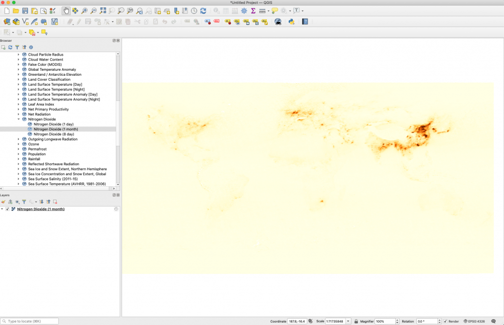
There are several datasets available for free that provide the country border and label for the world. I keep one handy in my directory that was created by Bjorn Sandvik at thematicmapping.org. Download your own copy here: https://thematicmapping.org/downloads/world_borders.php. Once you have downloaded and saved the file somewhere on your machine, unzip the file and drag and drop the TM_WORLD_BORDERS-0.3.shp into your QGIS window.
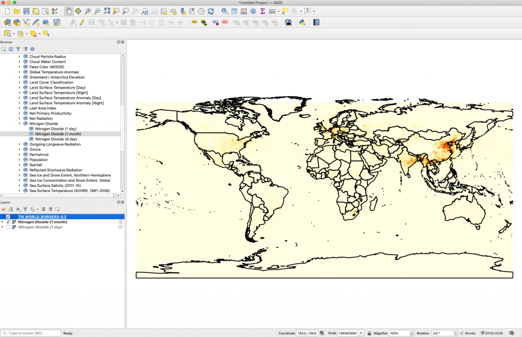
Now it is time to add labels.
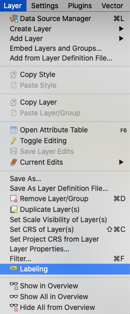
Go to Layer > Select Labeling and add Single Labels from the drop down in the Layer Styling window that pops up.
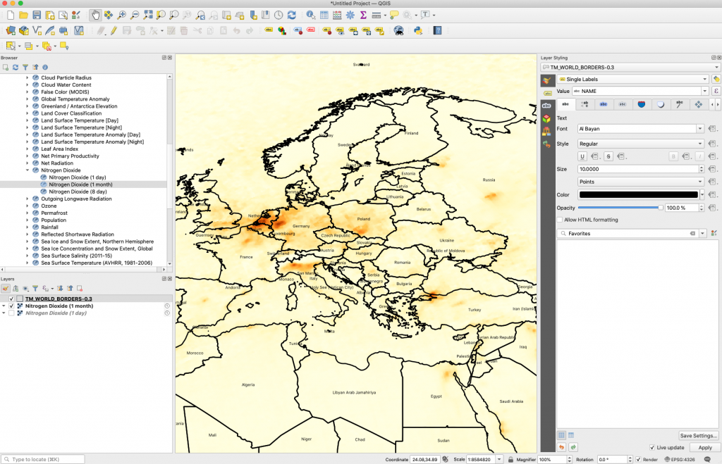
The map may not have the aesthetic you need to see the labels clearly. The color and font of the labels can be changed in the Layer Styling window. The color of the countries shapefile can be changed by double-clicking on the box next to the shapefile label in the Layers window.
If the labels do not provide the granularity needed for each country, try adding one of these shapefiles from the Centers for Disease Control and Prevention to your map using the same process: https://www.cdc.gov/epiinfo/support/downloads/shapefiles.html.
This blog has a few tips on choosing the right map color: https://neo.gsfc.nasa.gov/blog/2020/10/16/create-and-apply-the-right-color-palette-in-adobe-photoshop-for-your-map-visualization-part-1-of-3/.
Feel free to add any questions or tutorial suggestions in the comments below.
Comments Off on How To Add Country Labels to Your NEO Image
How to add NEO layers to your map using the NEO Web Mapping Service (WMS)
February 8th, 2021 by Andi Thomas
A Little Background Information on WMS
The Web Mapping Service (WMS) protocol has been around since 1999 and gives users the capability to access georeferenced maps via machine-to-machine contact. This means you can connect to a WMS server from a software of your choice that has WMS capabilities and load all or some of the datasets that are included on the WMS server you connect to.
There are a couple of required request types by a WMS server: GetMap and GetCapabilities. GetCapabilities provides information on what is available with a WMS service and GetMap provides the image map along with the image-specific metadata. NEO’s Capabilities Document is located on the WMS information page.
How to use the NEO WMS service
There are several ways to connect to NEO’s WMS server with different software. In fact, Wikipedia has a list of software with the WMS capability to explore. For this tutorial, we are going to use a free and open-source desktop geographic information system application called, QGIS. Assuming you have already installed QGIS on your machine, follow these simple steps to get started:
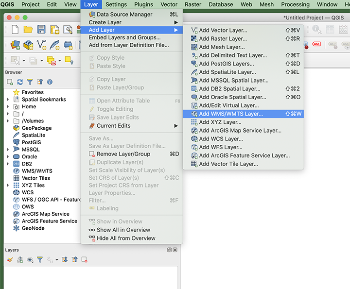
- Open a new QGIS project and go to Layer > Add Layer > Add WMS/ WMTS Layer…
- The Data Source Manager window should have popped up. Click New and the Create a New WMS/ WMTS Connection window will pop up.
- Fill in Name and URL:
- For Name, I am going to call it, “NASA Earth Observations“.
- The NEO WMS URL is: https://neo.gsfc.nasa.gov/wms/wms
- Click OK and you will see the NEO datasets populate in the Layers box.
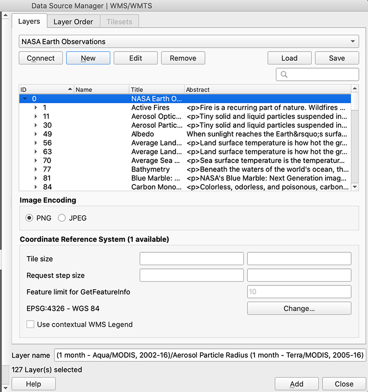
- You can Select the datasets you want to add to the map from here or, I prefer to close this window and add data to the map from the Browser window.
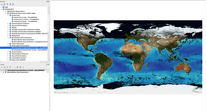
- From the Browser window, double-click a few of the datasets you would like to add to your map. I am going to add the Blue Marble basemap and the 1 month Chlorophyll Concentration Aqua/ MODIS dataset.
This is just a start to using the WMS service. There are plenty of other ways to use WMS capabilities as long as you have the URL (https://neo.gsfc.nasa.gov/wms/wms) and you know what datasets you want to use from the WMS service.
We would love to hear how you are using our WMS service. Please let us know in the comments below.
Comments Off on How to add NEO layers to your map using the NEO Web Mapping Service (WMS)
Raster and Floating Point GeoTIFFs: What is the difference?
December 23rd, 2020 by Andi Thomas
When you are considering which format to download for a NEO image, there are two GeoTIFF format options: GeoTIFF (raster) and GeoTIFF (floating point). This can be confusing at first. Let’s take a look at both examples using the Chlorophyll Concentration dataset to distinguish the two formats.
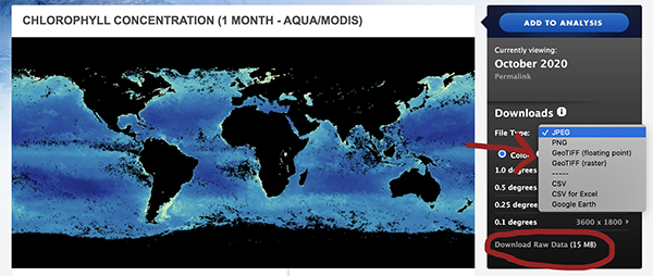
The image above is what downloads when you select GeoTIFF (floating point). This is a floating-point image file where each cell has a number with a decimal (ex. 1.1111). We call this format “data-like” for our purposes because it has been scaled and resampled as part of the processing of the original source data for NEO and the files are simplifications of the original data. Keep this in mind when you are using NEO imagery for analysis—our datasets should not be used for scientific research because they were not calibrated to the precision needed for scientific analysis. If you want to do your own processing for scientific research, choose the “Download Raw Data” option located in the Downloads box.
To simplify even further, the GeoTIFF (raster) above is an 8-bit color image. The values are stored as 8 bit grayscale and the color table is applied on-the-fly based on those values.
If you have any additional questions or need further clarification, please email us through the “Contact Us” button below.
Comments Off on Raster and Floating Point GeoTIFFs: What is the difference?
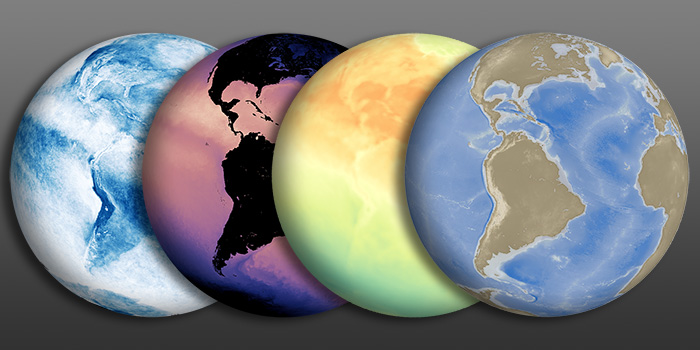
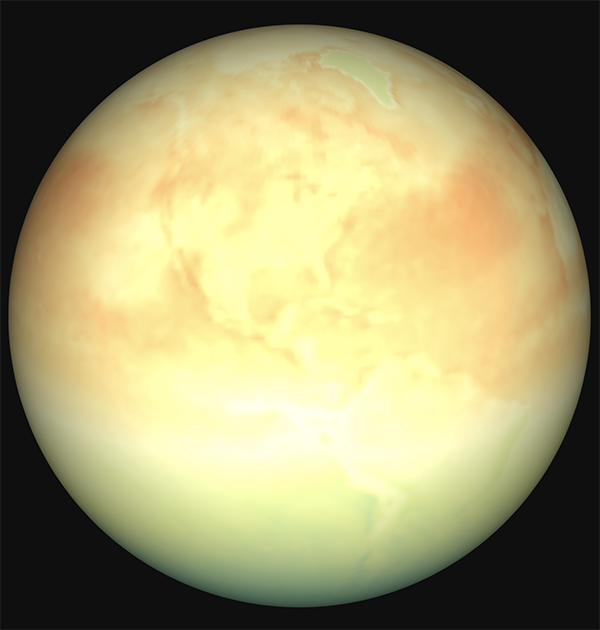
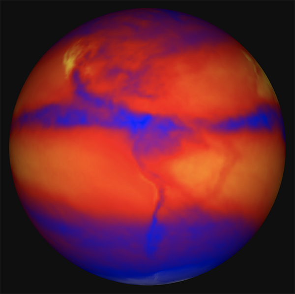
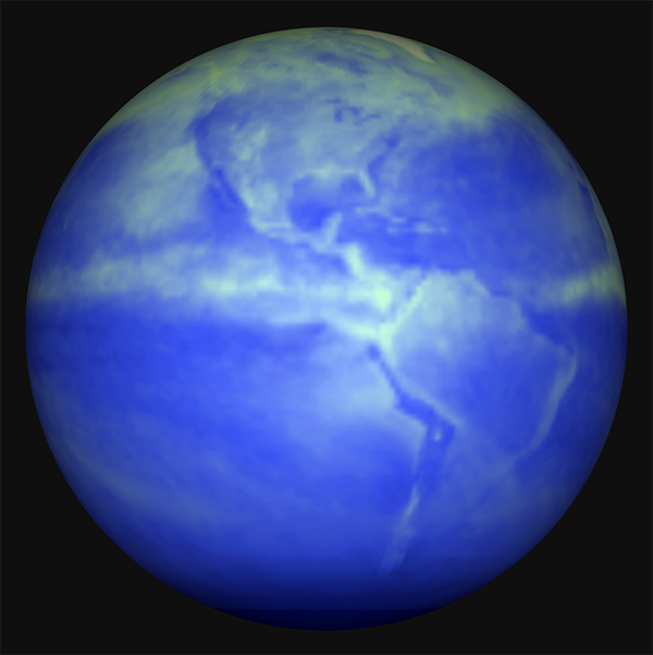
View NEO Imagery on a Sphere
November 23rd, 2020 by Andi Thomas
There are several companies and organizations that provide spherical projector technology, but the first one I had ever heard of was Science on a Sphere (SOS) created by the National Oceanic and Atmospheric Administration (NOAA). Originally envisioned in 1995 by Dr. Alexander “Sandy” MacDonald and later patented in 2005, these Science on a Spheres (and other variations) are in hundreds of locations across the United States and abroad to help increase understanding of Earth’s complex processes.
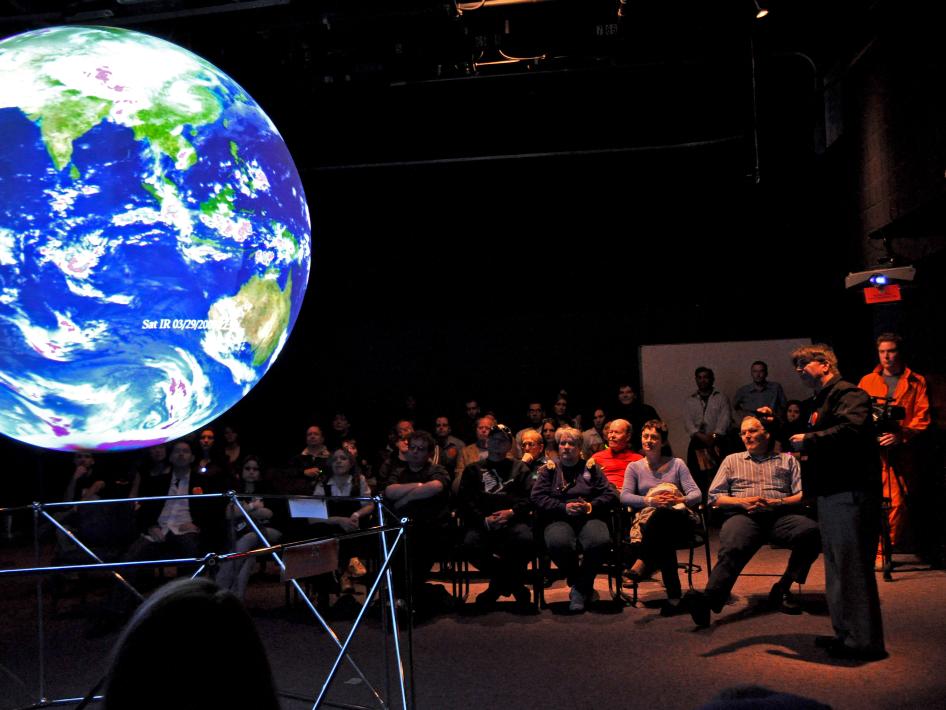
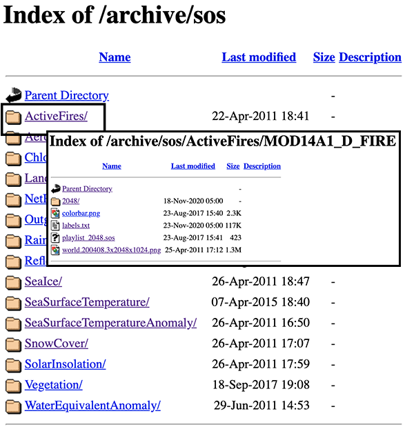
In support of these visualization systems, NEO provides an archive of time-lapse global imagery to display in spherical projections located in the NEO SOS Archive. NEO uses the Content Creation Guidelines by NOAA to provide a time series in the preferred projection, image format, and resolution. There is also a labels.txt file available with each dataset to label the images with the correct acquisition, a color bar file to provide context to each time series, and a PIP text file (.SOS) that points to the labels and color bar file along with extra features like fade in time and frame rate. Please see the SOS Remote App manual to learn how to display NEO’s time-series datasets on your display system using the SOS Remote App.
This service started based on requests and only has part of the NEO archive available. If you see a dataset that is not in the archive on our site and you would like it for your spherical visualization, please send us an email using the Contact Us link below.
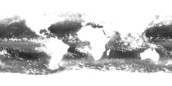
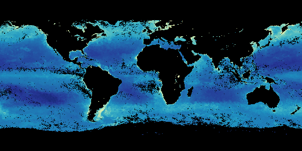
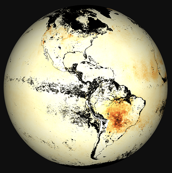
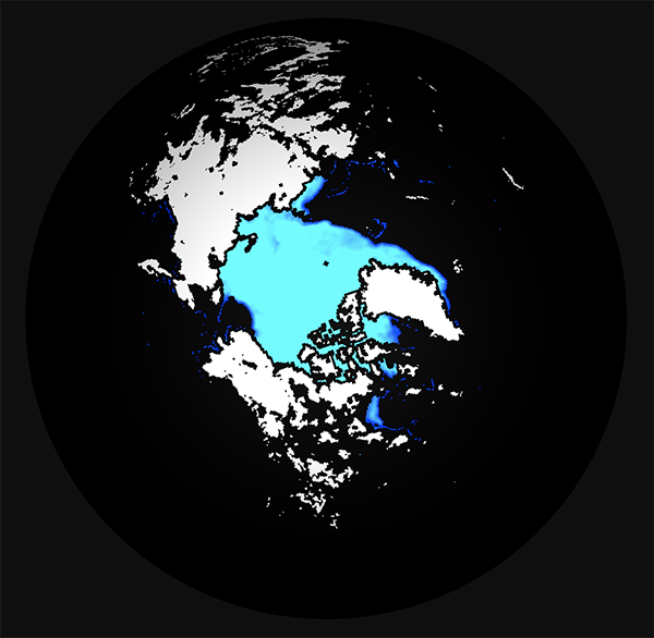
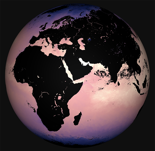
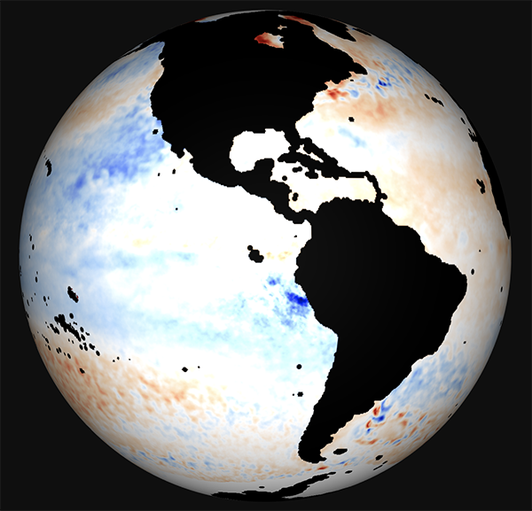
Here is a preview of some of the datasets we currently have available in the SOS Archive:
Active Fires from Terra/ MODIS
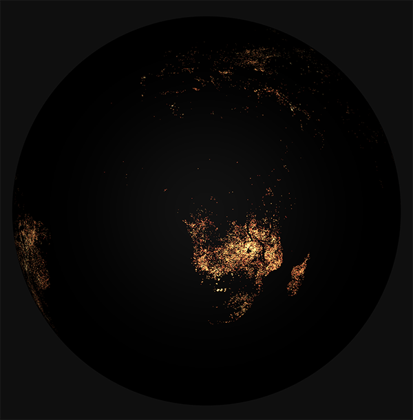
Aerosol Optical Thickness (Depth) from Terra/ MODIS
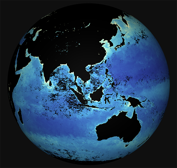
Chlorophyll Concentration from Aqua/ MODIS
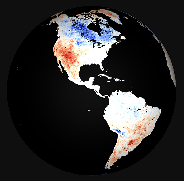
Land Surface Temperature Anomaly (Day) from MODIS
Net Radiation from CERES
Outgoing Longwave Radiation from CERES
Rainfall from TRMM
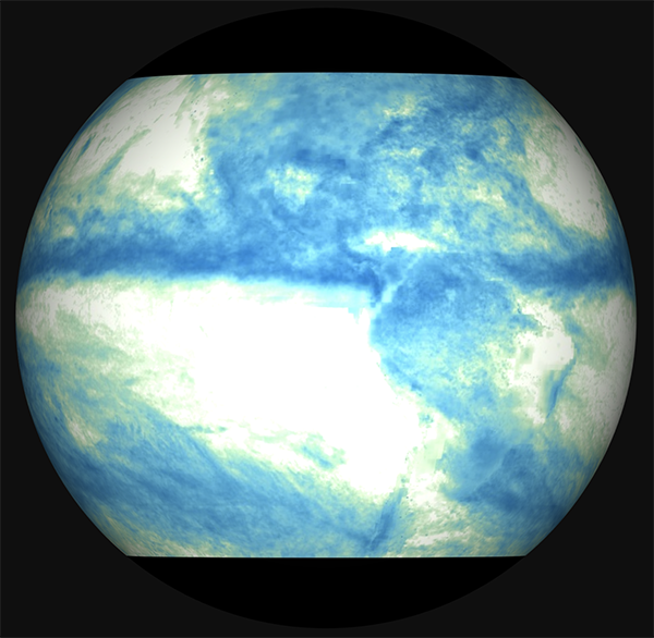
Reflected Shortwave Radiation from CERES
Sea Ice Concentration from SSM/I / DMSP
Sea Surface Temperature from Aqua/ MODIS
Sea Surface Temperature Anomaly from AQUA/AMSR-E
Comments Off on View NEO Imagery on a Sphere
Questions asked frequently at NEO
September 3rd, 2020 by Andi Thomas
After many years of serving the public with global visualizations of Earth’s system processes, we gathered the most frequent questions visitors of our site ask and answered them for you. The FAQs page can be found on the home page and lives here: https://neo.gsfc.nasa.gov/faq/. Please look these questions over and see if they answer questions you may have had already or discoveries that will help understand our site better.
If you read through the page and still have your own unanswered questions we did not cover, please send us an email using the contact form below and we will make sure you are heard.
Comments Off on Questions asked frequently at NEO
NEO FTP Service No Longer Available
June 13th, 2019 by Kevin Ward
Effective June 13, 2019, the NEO File Transfer Protocol (FTP) service is no longer available. It has been replaced with access via HTTPS.
Comments Off on NEO FTP Service No Longer Available
NEO FTP Service is Retiring
March 15th, 2019 by Kevin Ward
NASA is in the process of deprecating the use of FTP protocol for file access across the agency. As a result, downloading files from NEO via FTP may no longer be available after April 15, 2019. NEO will support bulk downloading options via HTTPS, but FTP client software applications will no longer be able to access NEO holdings. Similarly, if users are using FTP command line utilities or scripts to download from the archive, those will need to be converted to using HTTPS-access methods.
The directories containing the bulk files can be found at https://neo.gsfc.nasa.gov/archive/ Additionally, you may also use our Web Mapping Service (WMS).
For users who have scripts or command line experience, we recommend using either wget or curl to facilitate downloading from the bulk archive. There is quite a bit of documentation and examples that can be found simply by searching, or even just looking at the wget man page, but here are a couple wget examples:
If you want to maintain an up-to-date mirror of a specific directory, retrieving only the PNG files:
wget --no-directories --no-host-directories --no-parent --recursive --mirror --accept "*.PNG" -l1 https://neo.gsfc.nasa.gov/archive/rgb/MOD_LSTD_M/
Same as above, but get only the images from 2007 (for example):
wget --no-directories --no-host-directories --no-parent --recursive --mirror --accept "*2007*.PNG" -l1 https://neo.gsfc.nasa.gov/archive/rgb/MOD_LSTD_M/
If you are not comfortable using command line utilities to download NEO imagery, there is a growing number of graphical interfaces to facilitate downloading over HTTPS. Some are stand-alone applications, some are browser plugins. You can find these applications by searching on “download multiple files from website.”
Data-like File Formats: CSV and floating point GeoTIFFs
December 23rd, 2013 by Kevin Ward
In addition to the standard file formats that we support in NEO—JPEG, PNG, GeoTIFF, and GoogleEarth—many (not all) datasets support two additional “data-like” formats: CSV (comma-separated values) and floating point GeoTIFF. When you choose one of these formats for download, there are a few details that should be taken into consideration.
- The values that these files contain have been scaled and resampled for visualization purposes in NEO and should not be considered for rigorous scientific examination. At best they are useful for basic analysis and trend detection but if you are interested in conducting research-level science we recommend that you use the original source data (which are not hosted by NEO, but we can assist you in identifying the source).
- CSV files can get quite large at full resolution. For example, a 3600×1800 CSV file can get to around 61MB. If your software has difficulty opening a file of that size then please select a smaller resolution (e.g., 1440×720).
- There are two flavors of CSV available in NEO:
- “Regular” CSV which includes the text-only values at the resolution the user specifies. This format is suitable for Excel (2007 and later) and many other applications.
- “CSV for Excel” In Excel versions prior to 2007, worksheets could not support more than 256 columns. To remedy this, this format option is resized to 250×125. The first row contains the longitude values for the center of the cell and the first column contains the latitudes.
- Floating point GeoTIFFs contain 32-bit numerical data along with the geolocation information that is standard for the Geo format. These files can also get large as they are not internally compressed—e.g., a 3600×1800 GeoTIFF can be around 25MB.
These formats are not available by default in our archive but if you are interested in obtaining a long time series of a dataset in one of these formats, please contact us and we can perform a customized export to the ftp site in the format you need.
- Browse by Topic
- Analysis
- NEO in the Media
- New Datasets
- Services
- Uncategorized
- Browse by Date
- June 2026
- July 2025
- August 2024
- May 2023
- April 2021
- February 2021
- December 2020
- November 2020
- October 2020
- September 2020
- June 2019
- March 2019
- April 2015
- April 2014
- December 2013
- November 2013
- August 2013
- March 2013
- June 2012
- June 2011
- April 2011
- November 2010
- August 2010
- February 2009
- May 2008
- April 2007