Unfortunately, due to new NASA web requirements and diminishing resources, the NEO analysis tool will be removed from the site effective June 1, 2023. We apologize for the inconvenience this may cause. I encourage you to look at some other of our analysis-related blog posts to learn how to use NEO imagery in QGIS and Excel.

We recently received an email about adding country labels to a NEO image to better understand where certain data points are in the world. Here is one way to add labels to any NEO image in QGIS.

QGIS is a free and open-source Geographic Information System. If you do not have QGIS on your machine, there are copies available for download here: https://qgis.org/en/site/forusers/download.html.

Then, follow this blog to add NEO layers to your map via WMS in QGIS: https://neo.gsfc.nasa.gov/blog/2021/02/08/how-to-add-neo-layers-to-your-map-using-the-neo-web-mapping-service/.

We are now ready to add country labels to your NEO layer of choice. For this example, I am going to use the Nitrogen Dioxide (1 month) dataset.

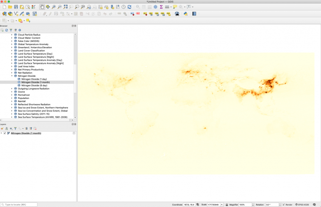
There are several datasets available for free that provide the country border and label for the world. I keep one handy in my directory that was created by Bjorn Sandvik at thematicmapping.org. Download your own copy here: https://thematicmapping.org/downloads/world_borders.php. Once you have downloaded and saved the file somewhere on your machine, unzip the file and drag and drop the TM_WORLD_BORDERS-0.3.shp into your QGIS window.

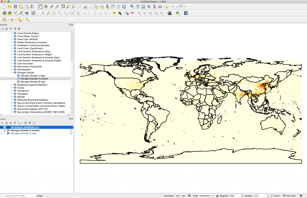
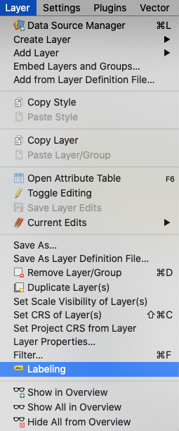
Now it is time to add labels.

Go to Layer > Select Labeling and add Single Labels from the drop down in the Layer Styling window that pops up.

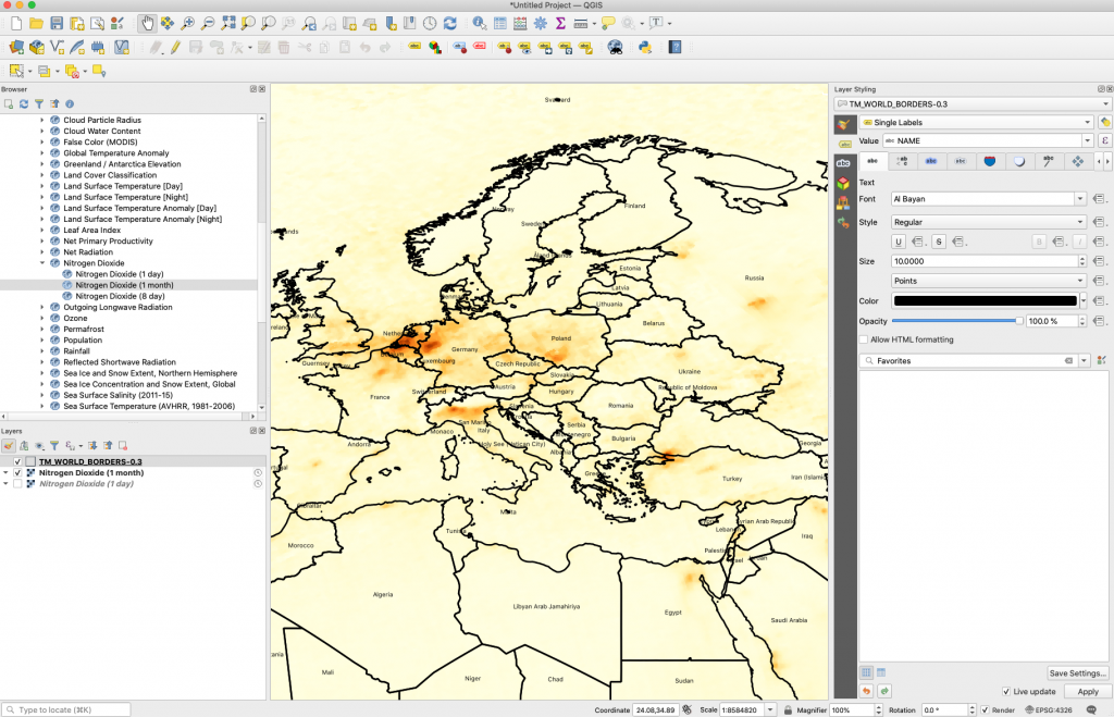
The map may not have the aesthetic you need to see the labels clearly. The color and font of the labels can be changed in the Layer Styling window. The color of the countries shapefile can be changed by double-clicking on the box next to the shapefile label in the Layers window.

If the labels do not provide the granularity needed for each country, try adding one of these shapefiles from the Centers for Disease Control and Prevention to your map using the same process: https://www.cdc.gov/epiinfo/support/downloads/shapefiles.html.

This blog has a few tips on choosing the right map color: https://neo.gsfc.nasa.gov/blog/2020/10/16/create-and-apply-the-right-color-palette-in-adobe-photoshop-for-your-map-visualization-part-1-of-3/.

Feel free to add any questions or tutorial suggestions in the comments below.

When you are considering which format to download for a NEO image, there are two GeoTIFF format options: GeoTIFF (raster) and GeoTIFF (floating point). This can be confusing at first. Let’s take a look at both examples using the Chlorophyll Concentration dataset to distinguish the two formats.

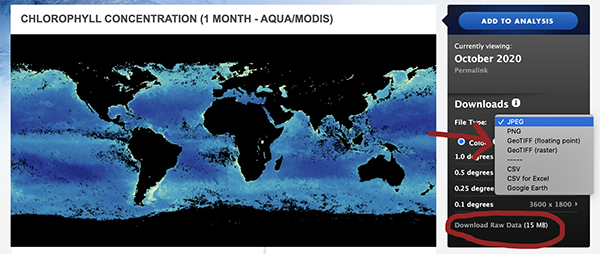
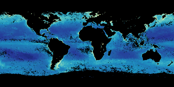
The image above is what downloads when you select GeoTIFF (floating point). This is a floating-point image file where each cell has a number with a decimal (ex. 1.1111). We call this format “data-like” for our purposes because it has been scaled and resampled as part of the processing of the original source data for NEO and the files are simplifications of the original data. Keep this in mind when you are using NEO imagery for analysis—our datasets should not be used for scientific research because they were not calibrated to the precision needed for scientific analysis.  If you want to do your own processing for scientific research, choose the “Download Raw Data” option located in the Downloads box.

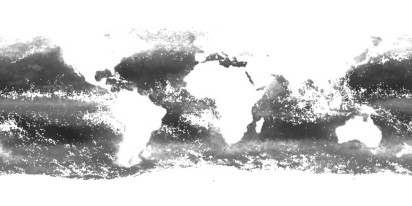
To simplify even further, the GeoTIFF (raster) above is an 8-bit color image. The values are stored as 8 bit grayscale and the color table is applied on-the-fly based on those values.

If you have any additional questions or need further clarification, please email us through the “Contact Us” button below.

We have added the NEO color table to a grayscale image, learned how to accommodate the color blind easily with our maps, and now we are ready to build custom color palettes.

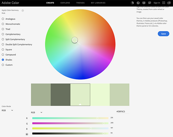
Adobe has an online color wheel that is helpful to use when surfing through different colors. If you are unsure what colors to start with, use the color wheel to give you a few ideas and follow these three steps as a guide for applying colors to your map with the wheel:

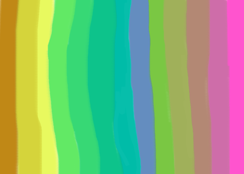
Step 1. Play around with the different color functions of the wheel to find a palette you would like to work with. You can work with a different hue and saturation of one color or look at three different complimentary colors. The radio buttons on the side of the wheel will help guide your decision-making. The RGB value for each color is at the bottom. Feel free to also mess with the lightness, hue and saturation sliders to get exactly what you want after the color wheel gives you an output. I decided to use the shades function and make a minty green palette. I plan to use these colors for land and then choose a contrasting color for the water.

Step 2. Open the color table back up for the grayscale image and use the same method as before: Select a couple of rows and change the colors to what you selected on the wheel, gradually moving from light to dark down the color table. Or, see what happens when you move from dark to light down the color table. Does it change the message of the map?

Step 3. Save your color palette for future use.

Alright, I know, that was short and easy. But not so fast, we have a couple more things to learn.

Follow these steps to make your own color palette in Photoshop:

Step 1. Open a new project for a clean slate to make palettes on. Do not worry about the canvas size as long as you have enough space to work with.

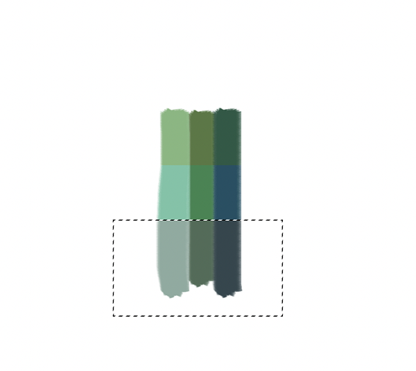
Step 2. Using the brush tool at a size that is easy to see, pick and paint a color on the canvas that you want on your map. I chose green because that is what I think of when I think of vegetation.

Step 3. Now open the Color Picker back up and select a color that is lighter (less saturated) and move the hue up the color scale a little bit. Repeat this process but in the other direction for your third color. There is a tutorial by Greg Gunn that has a very similar process but is way more detailed. Please check out the video if you need a little more context on choosing the right colors.

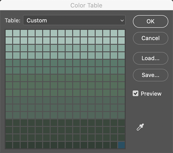
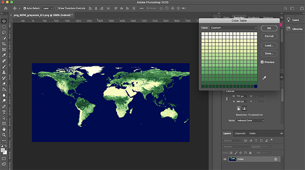
Step 4. I have chosen a few colors to work with and am ready to add them to the color table. Clip the canvas to the colors you would like on your map. Go to Image, Mode, and select Indexed Color. Now open up the Color Table under Image, Mode. The colors you have chosen may be scattered around the table.

Step 5. Select one of your lightest colors on the table and add it to the 5th and 6th rows using the RGB values located on Color Picker. I may choose to add the same colors to three rows instead of two but this is a good starting place.

Step 6. Create a lighter color from the one you just filled in the 5th and 6th rows by toggling hue and saturation in Color Picker and add it to the 3rd and 4th rows. Repeat this process for rows 1 and 2.

Step 7. Now pick a second color that is darker than rows 5 and 6 and add it to rows 7 and 8. Repeat this process all the way down.

Step 8. Choose and apply a contrasting color for the last cell to represent water.

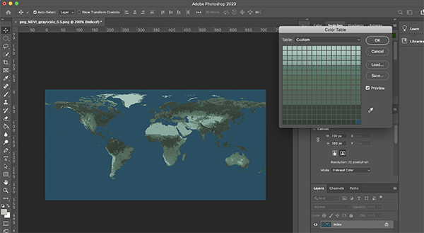
Step 9. Save the color table somewhere that is easy to find and open up a new project with the grayscale NDVI map.

Step 10. Change the mode to Indexed Color and open up the Color Table.

Step 11. Load the color table you just created and see what you think. Feel free to change the colors up or maybe even repeat the steps with an entirely new set of colors. This tutorial is not available to get it right on the first try. We simply want to give you the tools you need to make the right map for your needs.

Now that we have finished part one and understand how the color table provided with each dataset on NEO is applied to each grayscale map, let’s focus on creating custom color palettes that are easy for everyone to see.

Color-blindness is a common condition that prohibits some individuals (mostly men) from distinguishing between colors. Especially, red and green.

Luckily, there are plenty of resources that can help with creating color-blind friendly maps. Color Brewer is one great place to start for pairing colors together and we will use the site throughout this part of the series to guide our color decision-making.

Follow these steps to surf through Color Brewer and customize a color palette that suits your needs and the color-blind:

Step 1. Navigate to the Color Brewer site and make sure the colorblind safe box is selected.

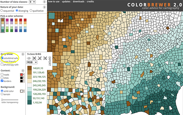
Step 2. Select 9 classes so you will have plenty of colors to work with for an 8-bit dataset. An 8-bit dataset has 256 values (0-255) which means the color table we are working with is a 16 x 16 grid. This will make more sense when we are looking at the color table in Photoshop. You could select 8 classes so every two rows have a different color, but I like to graduate the color to one row at the end. I encourage you to play around with a few combinations and decide what is best for your map.

Step 3. Instead of the default HEX codes, Select RGB from the drop down.

Step 4. Pick a color scheme. I am going to choose the yellow to green combo under sequential multi-hue. It is similar to what we are displaying now but lighter and I really want the water to be more of a dark blue rather than black.

Step 5. Go back to Photoshop and open the Color Table window again (Image, Mode, Color Table…). To make it easier, my Color Brewer window and Photoshop application are sitting side-by-side on my screen.

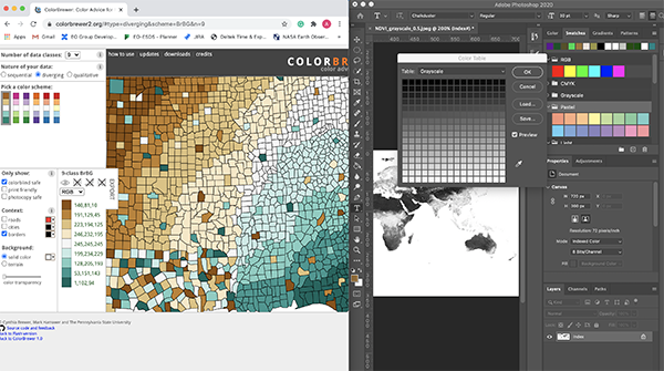
Step 6. Select two rows at a time on the color table and change the color using the RBG values that are on Color Brewer for the scheme you selected. Repeat this step as you move down the color bar until you get to the last two rows. Then you can graduate to one row and use the darker colors at the bottom of the scheme for the last two rows. The very last color (0) on the table is the map’s water (technically, it is areas of no data that are also where the oceans are). I chose to make the water a dark blue color rather than black.

Step 7. Save the color table you have created to load to another map if you like what you see.

Spend a little more time trying out different colors and using the options Color Brewer provides. Keep in mind, the map represents a dataset and in this case we are trying to show areas of less and more vegetation. Choose wisely on the colors you want to represent places with dense and sparse vegetation. Next time we will look at creating a custom color palette from scratch and applying it to your map.

Applying the right color palette to an image is crucial to conveying the right message to your audience. There are obvious no-nos in map-making like, do not color land and water blue because it may look like your entire map is water. Or, do not color a disaster map green because it may convey a message of positivity. This tutorial series will show you how to apply and save different color palettes, but it is important to look into why different colors are chosen, basic color theory, and best practices for choosing the right palette. There is a 6-part series on Earth Observatory published several years ago called the “Subtleties of Color” that is still a great base to start from before making and applying your own palettes. If you already feel comfortable with your knowledge and use of colors, let’s make color palettes!

Each NEO image is natively grayscale and the color table is applied in post-processing to display the colored image on each dataset’s page. Underneath the image is a downloadable Adobe Color Table (ACT) that can be saved and used to create and save color palettes for other grayscale images.

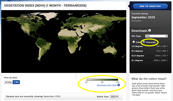
Let’s look at the Vegetation Index (NDVI) MODIS imagery as an example for applying a ready-made color table for the dataset following these steps:

Step 1. Download and save the color palette displayed for the NDVI imagery (filename: modis_ndvi.act) and a grayscale PNG at the temporal and spatial resolution of your choice. I saved the files to my desktop so they would be easy to find.

Step 2. Open Photoshop and load the grayscale NDVI image into a new project.

Step 3. Make sure the swatches window is open. There should be a check mark next to “Swatches” and the window should appear on the top right.

Step 4. In the swatches window, expand the hamburger button on the right and click Import Swatches

Step 5. Navigate to where you saved the ACT file and open the file. You should now see the color palette in the Swatches window under its filename and you will be able to access it later and even reuse some of the colors for your own palette creations.

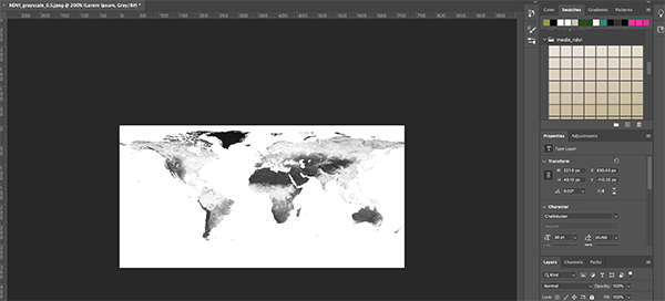
Step 6. Now go to Image, Mode, and select Indexed Color. Keep the default settings and click Ok. Your image name should have changed to “index”.

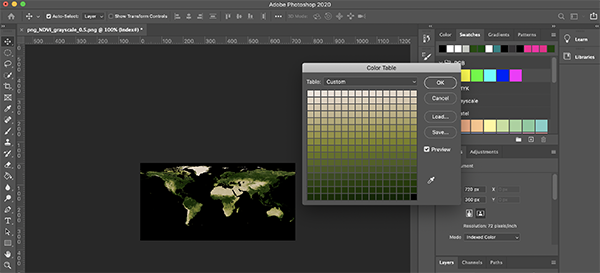
Step 7. Go back to Image, Mode and select Color Table…

Step 8. Select Custom from the drop-down menu at the top of the window and click Load…

Step 9. Navigate to the modis_ndvi.act file, select the file, and click Ok.

Step 10. The color applied to the map should now look the same as what is on our site for the MODIS Vegetation Index dataset.

Now we are ready to move on to part 2 where we will learn how to apply a custom color palette that is color-blind friendly. See you then!

Did you know you can use Excel to visualize raster datasets? If not, follow this short tutorial and find out how.

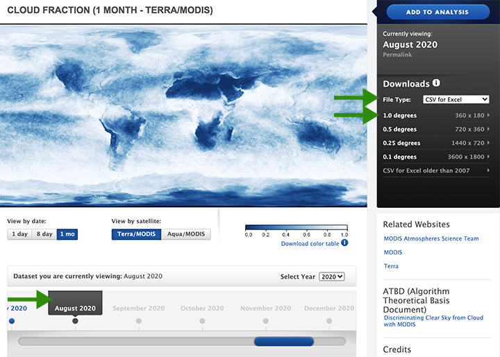
Let’s use the cloud fraction imagery NEO provides for this example.

Step 1. Go to the cloud fraction imagery page and choose the CSV for Excel download option from the drop-down at 1.0-degree resolution for a month and year of your choice. I am going to download the latest monthly image for August 2020.

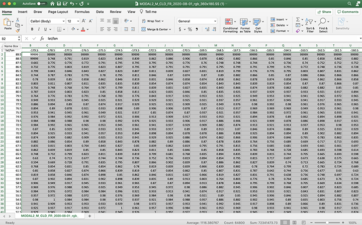
Step 2. Open the CSV in Excel and select all data except for the latitude and longitude row and column (which are the first row and first column).

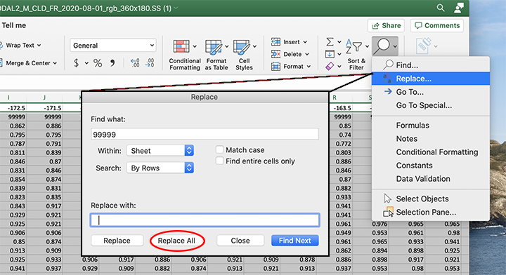
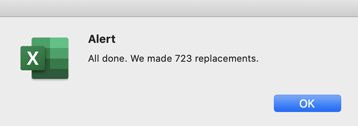
Step 3. Find and replace all 9999 values with an empty cell. I pressed the space bar a couple of times in the Replace with: cell. Once you click the Replace All button, an alert message will come up, and you will notice the cells that previously had 9999 are now empty.

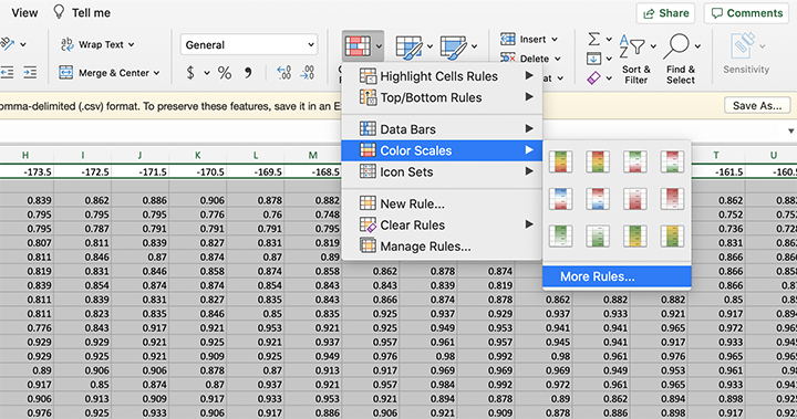
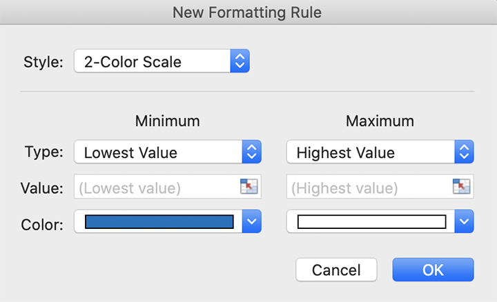
Step 4. From the Excel home tab: Select conditional formatting, color scales, and choose one of the 2-color scheme options available or select More Rules… and choose a different minimum and maximum value color. I am going to choose blue for the minimum color and white for the maximum color to create a look similar to what is available on the cloud fraction page.

Step 5. Zoom out using the slider on the bottom right side of the excel window and you will notice the global imagery taking shape.

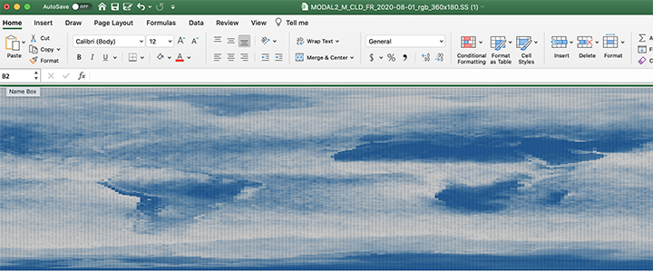
I remember learning the difference between raster and vector data in my entry-level GIS courses. Vector data is all of the point, line, and polygon data while raster data is made of cells or pixels. I wish my professor would have shown me how to visualize raster data in Excel at the time to really grasp cell values that make up the imagery we see as a whole. It certainly would have been easier to process!

Please share what you process in the comments below. We would love to hear any feedback or suggestions you may have.